Introduction to bayesAB

Most A/B test approaches are centered around frequentist hypothesis tests used to come up with a point estimate (probability of rejecting the null) of a hard-to-interpret value. Oftentimes, the statistician or data scientist laying down the groundwork for the A/B test will have to do a power test to determine sample size and then interface with a Product Manager or Marketing Exec in order to relay the results. This quickly gets messy in terms of interpretability. More importantly it is simply not as robust as A/B testing given informative priors and the ability to inspect an entire distribution over a parameter, not just a point estimate.

Enter Bayesian A/B testing.

Bayesian methods provide several benefits over frequentist methods in the context of A/B tests - namely in interpretability. Instead of p-values you get direct probabilities on whether A is better than B (and by how much). Instead of point estimates your posterior distributions are parametrized random variables which can be summarized any number of ways. Bayesian tests are also immune to ‘peeking’ and are thus valid whenever a test is stopped.

This document is meant to provide a brief overview of the bayesAB package with a few usage examples. A basic understanding of statistics (including Bayesian) and A/B testing is helpful for following along.

Methods

Unlike a frequentist method, in a Bayesian approach you first encapsulate your prior beliefs mathematically. This involves choosing a distribution over which you believe your parameter might lie. As you expose groups to different tests, you collect the data and combine it with the prior to get the posterior distribution over the parameter(s) in question. Mathematically, you are looking for P(parameter | data) which is a combination of the prior and posterior (the math, while relatively straightforward, is outside of the scope of this brief intro).

As mentioned above, there are several reasons to prefer Bayesian methods for A/B testing (and other forms of statistical analysis!). First of all, interpretability is everything. Would you rather say “P(A > B) is 10%”, or “Assuming the null hypothesis that A and B are equal is true, the probability that we would see a result this extreme in A vs B is equal to 3%”? I think I know my answer. Furthermore, since we get a probability distribution over the parameters of the distributions of A and B, we can say something such as “There is a 74.2% chance that A’s \(\lambda\) is between 3.7 and 5.9.” directly from the methods themselves.

Secondly, by using an informative prior we alleviate many common issues in regular A/B testing. For example, repeated testing is an issue in A/B tests. This is when you repeatedly calculate the hypothesis test results as the data comes in. In a perfect world, if you were trying to run a Frequentist hypothesis test in the most correct manner, you would use a power test calculation to determine sample size and then not peek at your data until you hit the amount of data required. Each time you run a hypothesis test calculation, you incur a probability of false positive. Doing this repeatedly makes the possibility of any single one of those ‘peeks’ being a false positive extremely likely. An informative prior, means that your posterior distribution should make sense any time you wish to look at it. If you ever look at the posterior distribution and think “this doesn’t look right!”, then you probably weren’t being fair with yourself and the problem when choosing priors.

Furthermore, an informative prior will help with the low base-rate problem (when the probability of a success or observation is very low). By indicating this in your priors, your posterior distribution will be far more stable right from the onset.

One criticism of Bayesian methods is that they are computationally slow or inefficient. bayesAB leverages the notion of conjugate priors to sample from analytical distributions very quickly (1e6 samples in <1s).

Usage Examples

We’ll walk through two examples. One Bernoulli random variable modeling click-through-rate onto a page, and one Poisson random variable modeling the number of selections one makes once on that page. We will also go over how to combine these into a more arbitrary random variable.

Bernoulli

Let’s say we are testing two versions of Page 1, to see the CTR onto Page 2. For this example, we’ll just simulate some data with the properties we desire.

library(bayesAB)

A_binom <- rbinom(250, 1, .25)
B_binom <- rbinom(250, 1, .2)

Of course, we can see the probabilities we chose for the example, but let’s say our prior knowledge tells us that the parameter p in the Bernoulli distribution should roughly fall over the .2-.3 range. Let’s also say that we’re very sure about this prior range and so we want to choose a pretty strict prior. The conjugate prior for the Bernoulli distribution is the Beta distribution. (?bayesTest for more info).

plotBeta(100, 200) # looks a bit off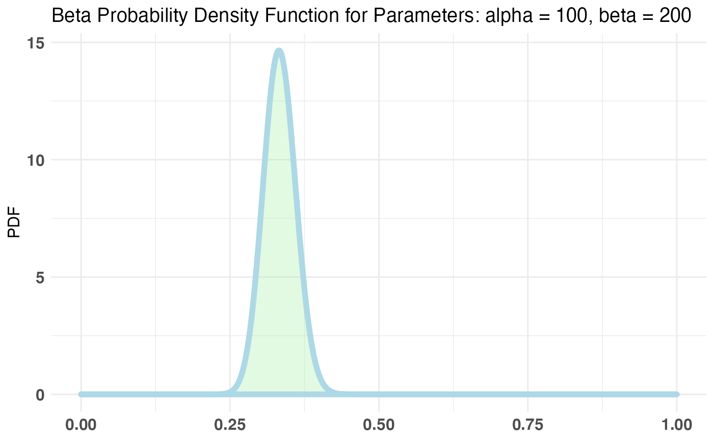

plotBeta(65, 200) # perfect

Now that we’ve settled on a prior, let’s fit our bayesTest object.

AB1 <- bayesTest(A_binom, B_binom, priors = c('alpha' = 65, 'beta' = 200), n_samples = 1e5, distribution = 'bernoulli')

bayesTest objects come coupled with print, plot and summary generics. Let’s check them out:

print(AB1)

## --------------------------------------------
## Distribution used: bernoulli 
## --------------------------------------------
## Using data with the following properties: 
##            A     B
## Min.    0.00 0.000
## 1st Qu. 0.00 0.000
## Median  0.00 0.000
## Mean    0.26 0.264
## 3rd Qu. 1.00 1.000
## Max.    1.00 1.000
## --------------------------------------------
## Conjugate Prior Distribution: Beta 
## Conjugate Prior Parameters: 
## $alpha
## [1] 65
## 
## $beta
## [1] 200
## 
## --------------------------------------------
## Calculated posteriors for the following parameters: 
## Probability 
## --------------------------------------------
## Monte Carlo samples generated per posterior: 
## [1] 1e+05

summary(AB1)

## Quantiles of posteriors for A and B:
## 
## $Probability
## $Probability$A
##        0%       25%       50%       75%      100% 
## 0.1737375 0.2392704 0.2520579 0.2652263 0.3475296 
## 
## $Probability$B
##        0%       25%       50%       75%      100% 
## 0.1754024 0.2412992 0.2540385 0.2672577 0.3377265 
## 
## 
## --------------------------------------------
## 
## P(A > B) by (0)%: 
## 
## $Probability
## [1] 0.47148
## 
## --------------------------------------------
## 
## Credible Interval on (A - B) / B for interval length(s) (0.9) : 
## 
## $Probability
##         5%        95% 
## -0.1687838  0.1836579 
## 
## --------------------------------------------
## 
## Posterior Expected Loss for choosing A over B:
## 
## $Probability
## [1] 0.05035903

plot(AB1)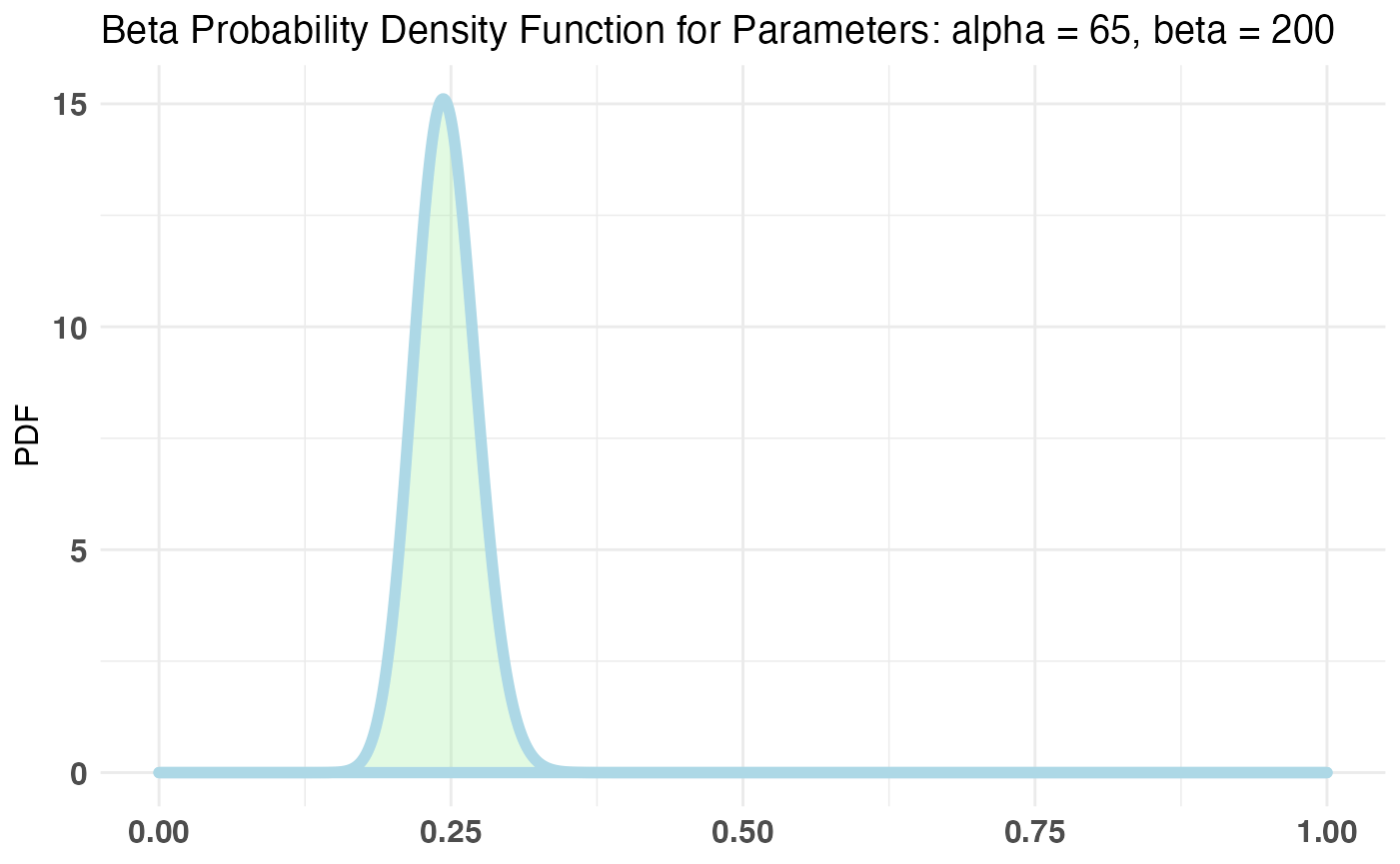

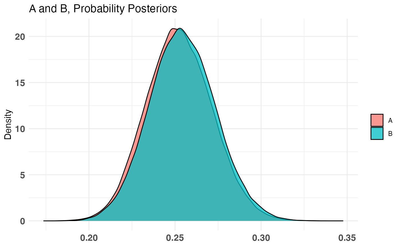
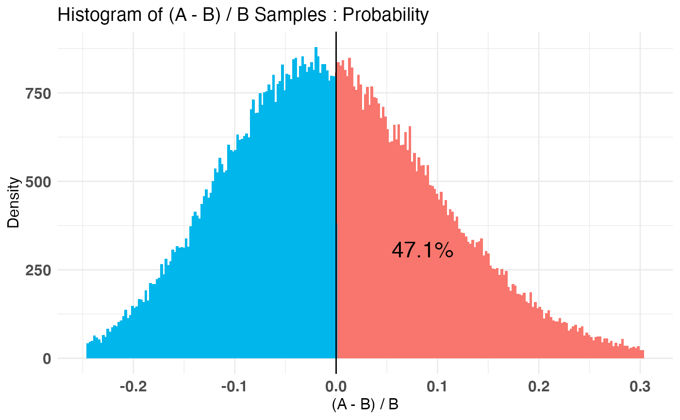
print talks about the inputs to the test, summary will do a P((A - B) / B > percentLift) and credible interval on (A - B) / B calculation, and plot will plot the priors, posteriors, and the Monte Carlo ‘integrated’ samples.

Poisson

Now we are on Page 2. On Page 2 you have any number of ‘interactions’ you can make (being vague is fun). Let’s say we wish to parametrize the amount of ‘interactions’ a user has by the Poisson distribution. Let’s also say, our priors would have us believe that the bulk of users will make between 5-6 interactions but we aren’t too sure on that number so we will allow a reasonable probability for other values. The conjugate prior for the Poisson distribution is the Gamma distribution.

A_pois <- rpois(250, 6.5)
B_pois <- rpois(250, 5.5)

plotGamma(30, 5) # 5-6 seem likely enough

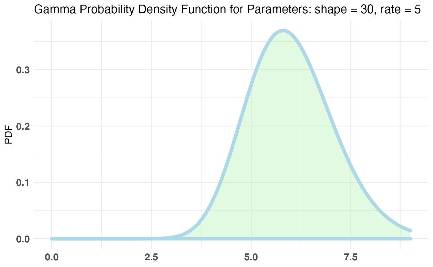
Let’s fit our bayesTest object in a similar manner.

AB2 <- bayesTest(A_pois, B_pois, priors = c('shape' = 30, 'rate' = 5), n_samples = 1e5, distribution = 'poisson')

print(AB2)

## --------------------------------------------
## Distribution used: poisson 
## --------------------------------------------
## Using data with the following properties: 
##              A      B
## Min.     1.000  1.000
## 1st Qu.  5.000  4.000
## Median   6.000  6.000
## Mean     6.428  5.672
## 3rd Qu.  8.000  7.000
## Max.    14.000 14.000
## --------------------------------------------
## Conjugate Prior Distribution: Gamma 
## Conjugate Prior Parameters: 
## $shape
## [1] 30
## 
## $rate
## [1] 5
## 
## --------------------------------------------
## Calculated posteriors for the following parameters: 
## Lambda 
## --------------------------------------------
## Monte Carlo samples generated per posterior: 
## [1] 1e+05

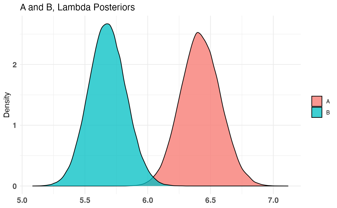
summary(AB2)

## Quantiles of posteriors for A and B:
## 
## $Lambda
## $Lambda$A
##       0%      25%      50%      75%     100% 
## 5.754699 6.312892 6.418301 6.527140 7.116775 
## 
## $Lambda$B
##       0%      25%      50%      75%     100% 
## 5.084133 5.577414 5.676565 5.777905 6.340495 
## 
## 
## --------------------------------------------
## 
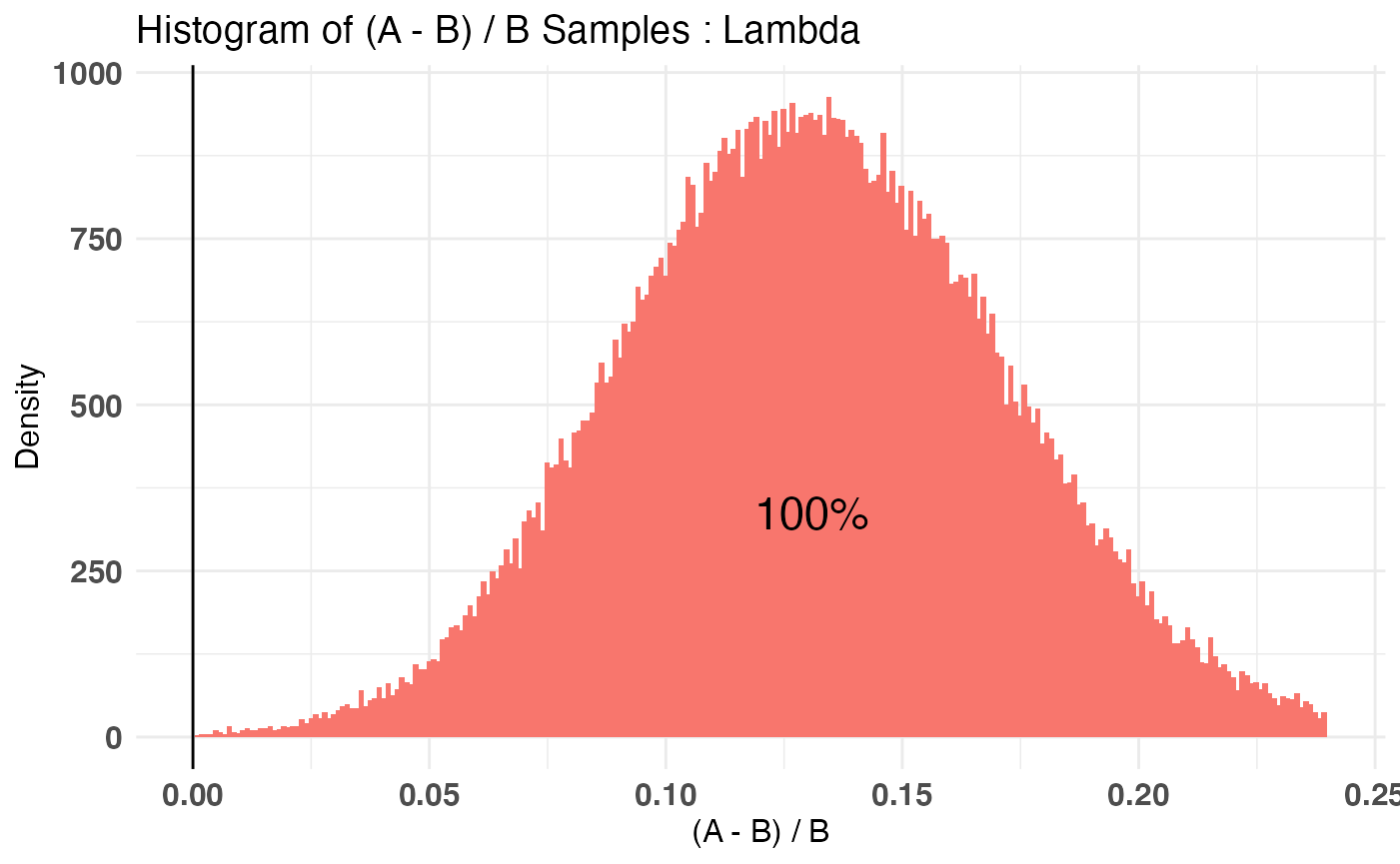
## P(A > B) by (0)%: 
## 
## $Lambda
## [1] 0.9996
## 
## --------------------------------------------
## 
## Credible Interval on (A - B) / B for interval length(s) (0.9) : 
## 
## $Lambda
##         5%        95% 
## 0.06602483 0.19968813 
## 
## --------------------------------------------
## 
## Posterior Expected Loss for choosing A over B:
## 
## $Lambda
## [1] 3.03496e-06

plot(AB2)

Combining Distribution

Another feature of bayesAB is the ability to decompose your end distribution into a series of intermediate distributions which are easier to parametrize. For example, let’s take the above example and say we want to test the effect of JUST Page 1 on Page 2’s interactions. Sure, we can try to come up with a way to parametrize the behaviors on Page 2 in the context of the conversion from Page 1, but isn’t it easier to encapsulate both parts as their own random variables, with their own informed priors from past traffic data. Using the combine function in bayesAB we can make this possible. Let’s consider the same test objects we have already fit. A combined object would look like this:

AB3 <- combine(AB1, AB2, f = `*`, params = c('Probability', 'Lambda'), newName = 'Expectation')

# also equivalent with %>% if you like piping
library(magrittr)

AB3 <- AB1 %>%
  combine(AB2, f = `*`, params = c('Probability', 'Lambda'), newName = 'Expectation')

Small note: the magrittr example may not look very elegant but it comes in handy when chaining together more than just 2 bayesTests.

For the combined distribution, we use the * function (multiplication) since each value of the Poisson distribution for Page 2 is multiplied by the corresponding probability of landing on Page 2 from Page 1 in the first place. The resulting distribution can be thought of as the ‘Expected number of interactions on Page 2’ so we have chosen the name ‘Expectation’. The class of bayesTest is idempotent under combine, meaning the resulting object is also a bayesTest. That means the same generics apply.

print(AB3)

## --------------------------------------------
## Distribution used: combined 
## --------------------------------------------
## Using data with the following properties: 
##            A      A     B      B
## Min.    0.00  1.000 0.000  1.000
## 1st Qu. 0.00  5.000 0.000  4.000
## Median  0.00  6.000 0.000  6.000
## Mean    0.26  6.428 0.264  5.672
## 3rd Qu. 1.00  8.000 1.000  7.000
## Max.    1.00 14.000 1.000 14.000
## --------------------------------------------
## Conjugate Prior Distribution:  
## Conjugate Prior Parameters: 
## [1] "Combined distributions have no priors. Inspect each element separately for details."
## --------------------------------------------
## Calculated posteriors for the following parameters: 
## Expectation 
## --------------------------------------------
## Monte Carlo samples generated per posterior: 
## [1] 1e+05

summary(AB3)

## Quantiles of posteriors for A and B:
## 
## $Expectation
## $Expectation$A
##       0%      25%      50%      75%     100% 
## 1.069876 1.531765 1.617185 1.706365 2.225990 
## 
## $Expectation$B
##       0%      25%      50%      75%     100% 
## 1.012562 1.365511 1.442075 1.521204 1.961537 
## 
## 
## --------------------------------------------
## 
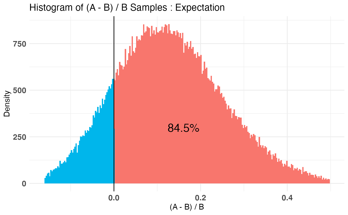
## P(A > B) by (0)%: 
## 
## $Expectation
## [1] 0.84481
## 
## --------------------------------------------
## 
## Credible Interval on (A - B) / B for interval length(s) (0.9) : 
## 
## $Expectation
##          5%         95% 
## -0.06932275  0.35149809 
## 
## --------------------------------------------
## 
## Posterior Expected Loss for choosing A over B:
## 
## $Expectation
## [1] 0.009674581

plot(AB3)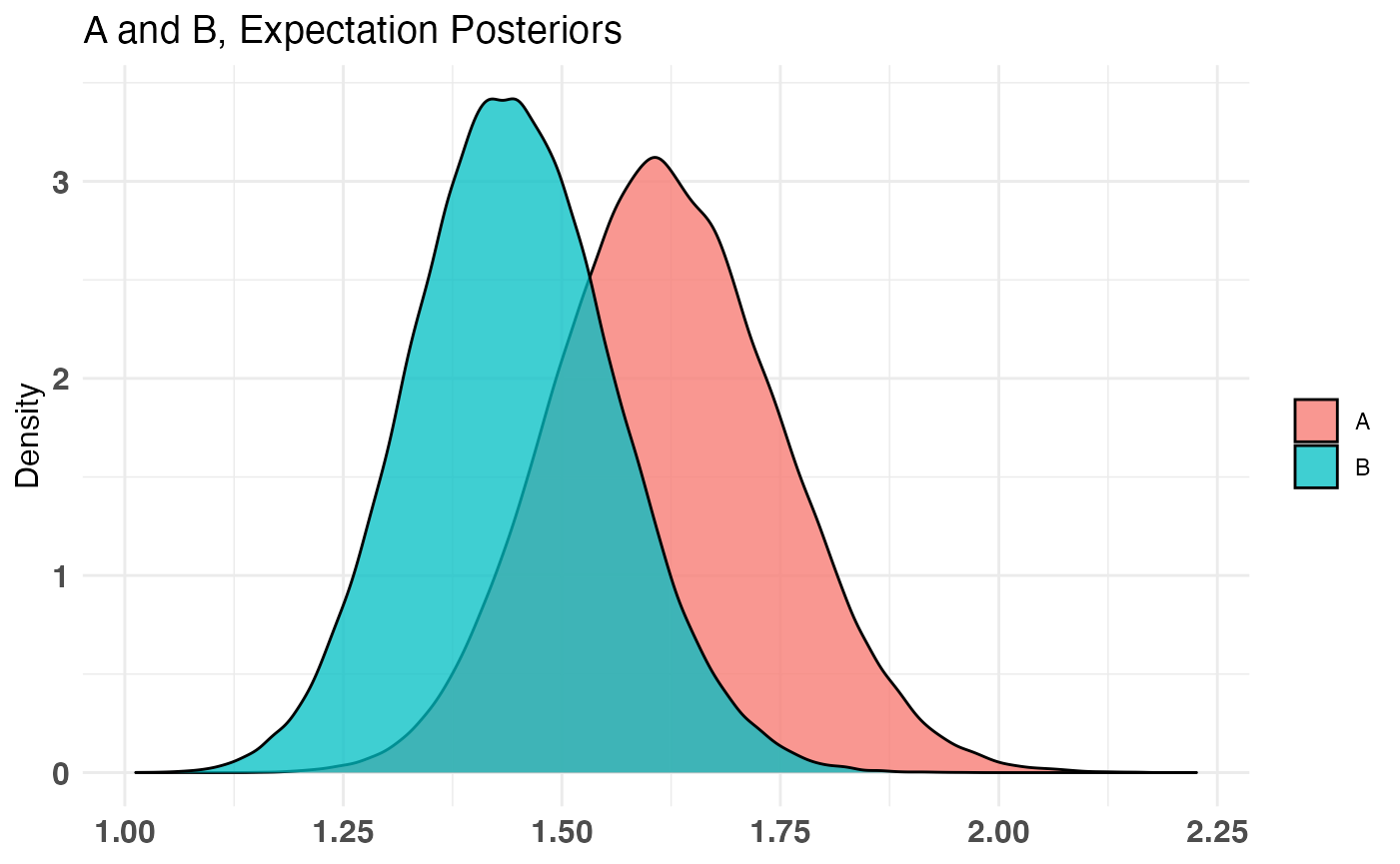

Conclusion

This document was meant to be a quick-start guide to A/B testing in a Bayesian light using the bayesAB package. Feel free to read the help documents for the individual functions shown above (some have default params that can be changed, including the generics). Report any issues or grab the development version from our Github.