Combine two (or any number, in succession) bayesTest objects into a new arbitrary posterior distribution.
The resulting object is of the same class.
combine(bT1, bT2, f = `+`, params, newName)
Arguments
| bT1 | a bayesTest object |
|---|---|
| bT2 | a bayesTest object |
| f | a binary function (f(x, y)) used to combine posteriors from bT1 to bT2 |
| params | a character vector of length 2, corresponding to names of the posterior parameters you want to combine; defaults to first posterior parameter if not supplied |
| newName | a string indicating the name of the new 'posterior' in the resulting object; defaults to string representation of f(params[1], params[2]) |
Value
a bayesTest object with the newly combined posterior samples.
Note
The generics `+.bayesTest`, `*.bayesTest`, `-.bayesTest`, and `/.bayesTest` are shorthand for combine(f = `+`), combine(f = `*`), combine(f = `-`), and combine(f = `/`).
See also
Examples
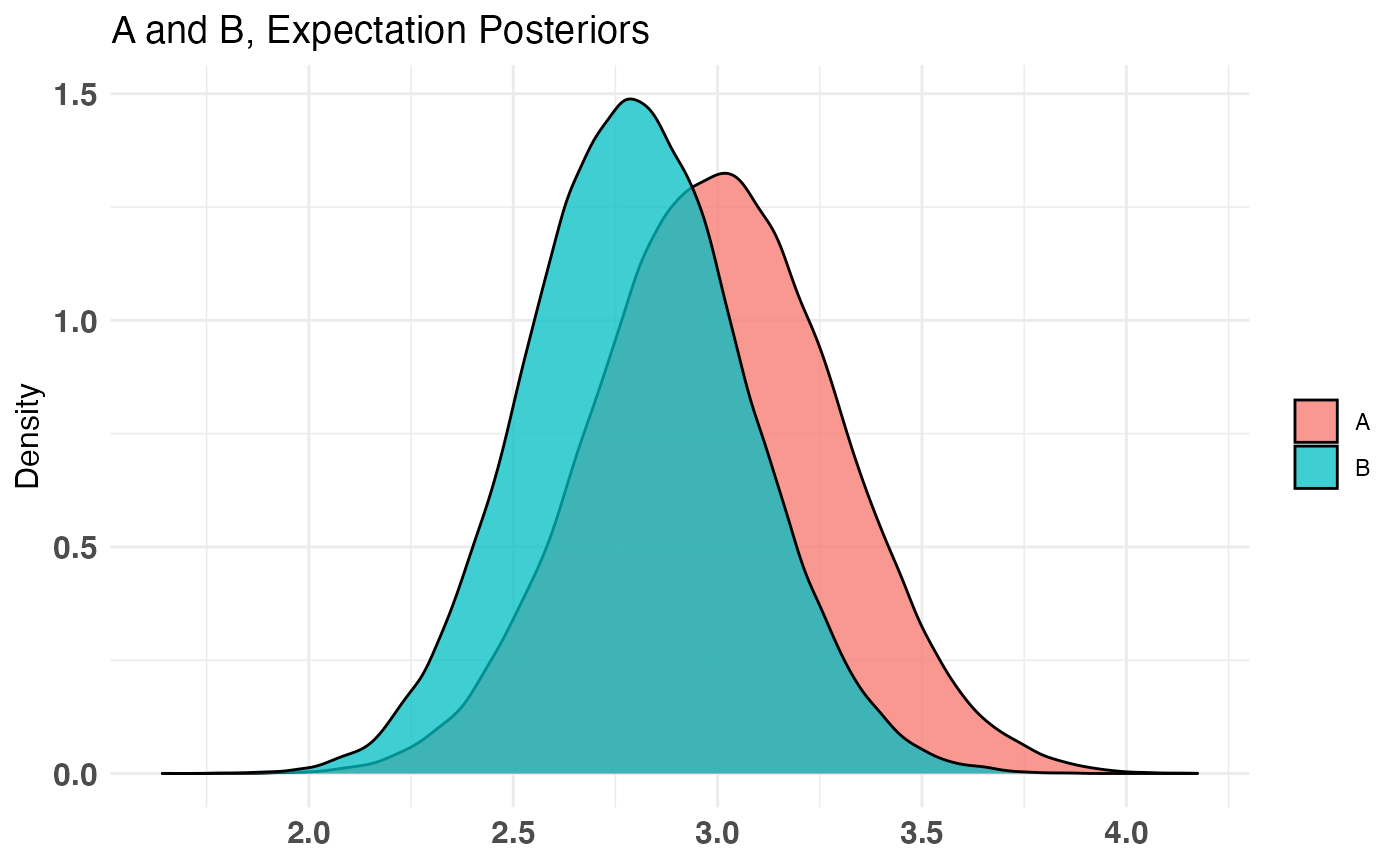
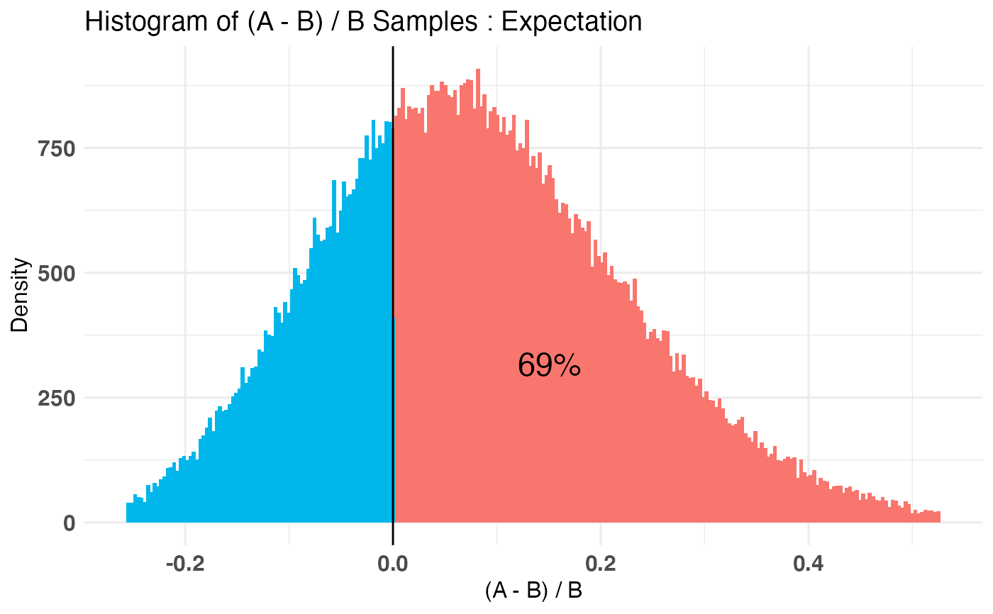
A_binom <- rbinom(100, 1, .5) B_binom <- rbinom(100, 1, .6) A_norm <- rnorm(100, 6, 1.5) B_norm <- rnorm(100, 5, 2.5) AB1 <- bayesTest(A_binom, B_binom, priors = c('alpha' = 1, 'beta' = 1), distribution = 'bernoulli') AB2 <- bayesTest(A_norm, B_norm, priors = c('mu' = 5, 'lambda' = 1, 'alpha' = 3, 'beta' = 1), distribution = 'normal') AB3 <- combine(AB1, AB2, f = `*`, params = c('Probability', 'Mu'), newName = 'Expectation') # Equivalent to AB3 <- AB1 * grab(AB2, 'Mu') # To get the same posterior name as well AB3 <- rename(AB3, 'Expectation') # Dummy example weirdVariable <- (AB1 + AB2) * (AB2 / AB1) weirdVariable <- rename(weirdVariable, 'confusingParam') print(AB3)#> -------------------------------------------- #> Distribution used: combined #> -------------------------------------------- #> Using data with the following properties: #> A A B B #> Min. 0.00 2.496988 0.00 -0.7000497 #> 1st Qu. 0.00 4.942534 0.00 2.8364165 #> Median 1.00 5.717172 1.00 4.2601330 #> Mean 0.51 5.888762 0.61 4.6022335 #> 3rd Qu. 1.00 6.898150 1.00 6.2211877 #> Max. 1.00 10.122432 1.00 13.6449519 #> -------------------------------------------- #> Conjugate Prior Distribution: #> Conjugate Prior Parameters: #> [1] "Combined distributions have no priors. Inspect each element separately for details." #> -------------------------------------------- #> Calculated posteriors for the following parameters: #> Expectation #> -------------------------------------------- #> Monte Carlo samples generated per posterior: #> [1] 1e+05#> Quantiles of posteriors for A and B: #> #> $Expectation #> $Expectation$A #> 0% 25% 50% 75% 100% #> 1.779334 2.796138 2.996819 3.198377 4.174025 #> #> $Expectation$B #> 0% 25% 50% 75% 100% #> 1.641447 2.618169 2.796646 2.978574 3.875928 #> #> #> -------------------------------------------- #> #> P(A > B) by (0)%: #> #> $Expectation #> [1] 0.68981 #> #> -------------------------------------------- #> #> Credible Interval on (A - B) / B for interval length(s) (0.9) : #> #> $Expectation #> 5% 95% #> -0.1498444 0.3428849 #> #> -------------------------------------------- #> #> Posterior Expected Loss for choosing A over B: #> #> $Expectation #> [1] 0.03028326 #>